[CS231n] 5. Neural Networks Part 1: Setting up the Architecture

keywords : model of a biological neuron, activation functions, neural net architecture, representational power

 

1) Biological motivation and connections

basic computational unit of the brain is a neuron

A cartoon drawing of a biological neuron (left) and its mathematical model (right).

 

• Model the firing rate of the neuron with an activation function f, which represents the frequency of the spikes along the axon.
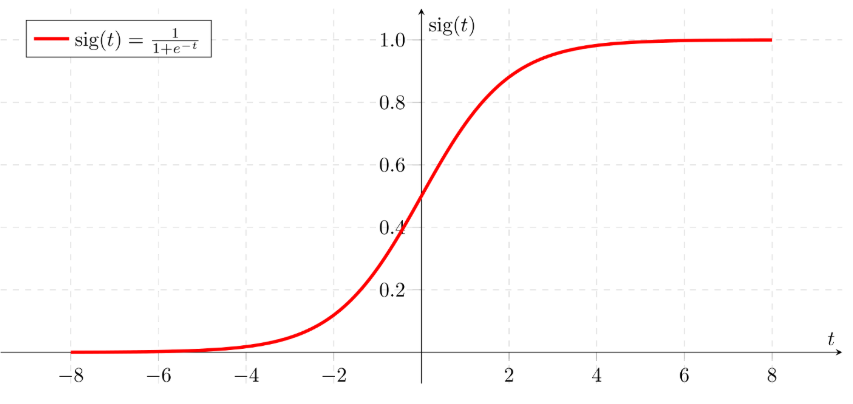
• Historically, a common choice of activation function is the sigmoid function σ, since it takes a real-valued input (the signal strength after the sum) and squashes it to range between 0 and 1

 

• Example code for forward-propagating a single neuron

class Neuron(object):
  # ... 
  def forward(self, inputs):
    """ assume inputs and weights are 1-D numpy arrays and bias is a number """
    cell_body_sum = np.sum(inputs * self.weights) + self.bias
    firing_rate = 1.0 / (1.0 + math.exp(-cell_body_sum)) # sigmoid activation function
    return firing_rate

• Each neuron performs a dot product with the input and its weights, adds the bias and applies the non-linearity (or activation function)

 

---

 

2) Single neuron as a linear classifier

As we saw with linear classifiers, a neuron has the capacity to “like” (activation near one) or “dislike” (activation near zero) certain linear regions of its input space.

• With an appropriate loss function on the neuron’s output, we can turn a single neuron into a linear classifier:

 

2.1) Binary Softmax classifier (a.k.a. Logistic Regression)

We can interpret σ(∑_i(w_ix_i+b)) to be the probability of one of the classes P(y_i=1∣ x_i;w)

The probability of the other class would be P(y_i=0∣x_i;w)=1−P(y_i=1∣x_i;w)

• Since the sigmoid function is restricted to be between 0-1, the predictions of this classifier are based on whether the output of the neuron is greater than 0.5.

sigmoid function

 

2.2) Binary SVM classifier

We could attach a max-margin hinge loss to the output of the neuron and train it to become a binary Support Vector Machine.

 

2.3) Regularization interpretation

The regularization loss in both SVM/Softmax cases could in this biological view be interpreted as gradual forgetting.

→ Since it would have the effect of driving all synaptic weights w towards zero after every parameter update.

📌  A single neuron can be used to implement a binary classifier (e.g. binary Softmax or binary SVM classifiers)

 

---

 

3) Commonly used activation functions

Every activation function (or non-linearity) takes a single number and performs a certain fixed mathematical operation on it.

 

3.1) Sigmoid

• It takes a real-valued number and “squashes” it into range between 0 and 1.
  → Large negative numbers become 0 and large positive numbers become 1.
  
  
• It has a nice interpretation as the firing rate of a neuron
  → From not firing at all (0) to fully-saturated firing at an assumed maximum frequency (1).

• In practice, the sigmoid non-linearity has recently fallen out of favor and it is rarely ever used. It has drawbacks
  1. Sigmoids saturate and kill gradients.
     Activation saturates at either tail of 0 or 1, the gradient at these regions is almost zero.
     → If the local gradient is very small, it will effectively “kill” the gradient and almost no signal will flow through the neuron to its weights and recursively to its data.
     → If the initial weights are too large then most neurons would become saturated and the network will barely learn.
  2. Sigmoid outputs are not zero-centered.
     Data that is not zero-centered has implications on the dynamics during gradient descent
     → If the data coming into a neuron is always positive (e.g. x>0 elementwise in f=wTx+b)), then the gradient on the weights w will during backpropagation become either all be positive, or all negative 
  3. exp() is a bit compute expensive
     
     

3.2) Tanh

• It squashes a real-valued number to the range [-1, 1].
• Its activations saturate, but unlike the sigmoid neuron its output is zero-centered.
  →In practice the tanh non-linearity is always preferred to the sigmoid nonlinearity.

3.3) ReLU

• It computes the function f(x) = max(0,x).

Pros

• It was found to greatly accelerate the convergence of stochastic gradient descent compared to the sigmoid/tanh functions.
  → It is argued that this is due to its linear, non-saturating form.
• Compared to tanh/sigmoid neurons that involve expensive operations (exponentials, etc.), ReLU can be implemented by simply thresholding a matrix of activations at zero. (Computationally efficient)

Cons

• ReLU units can be fragile during training and can “die”.→ With a proper setting of the learning rate this is less frequently an issue.
  → ReLU units can irreversibly die during training since they can get knocked off the data manifold.

 

3.4) Leaky ReLU

One attempt to fix the “dying ReLU” problem.

α is a small constant.

• Some people report success with this form of activation function, but the results are not always consistent.

 

3.5) Maxout

• Both ReLU and Leaky ReLU are a special case of this form (for example, for ReLU we have w1, b1=0).
  → The Maxout neuron therefore enjoys all the benefits of a ReLU unit (linear regime of operation, no saturation) and does not have its drawbacks (dying ReLU).
• It doubles the number of parameters for every single neuron, leading to a high total number of parameters.

“What neuron type should I use?”

Use the ReLU non-linearity, be careful with your learning rates and possibly monitor the fraction of “dead” units in a network. If this concerns you, give Leaky ReLU or Maxout a try. Never use sigmoid. Try tanh, but expect it to work worse than ReLU/Maxout.

 

---

 

4) Neural Network architectures

 

4.1) Layer-wise organization

Neural Networks are modeled as collections of neurons that are connected in an acyclic graph.

• Neural Network models are often organized into distinct layers of neurons.
• the most common layer type is the fully-connected layer
  → neurons between two adjacent layers are fully pairwise connected, but neurons within a single layer share no connections.

Left: A 2-layer Neural Network (one hidden layer of 4 neurons (or units) and one output layer with 2 neurons), and three inputs. Right: A 3-layer neural network with three inputs, two hidden layers of 4 neurons each and one output layer.

Notice that in both cases there are connections (synapses) between neurons across layers, but not within a layer.

 

4.2) Naming conventions

• N-layer neural network, we do not count the input layer.
• A single-layer neural network describes a network with no hidden layers (input directly mapped to output).
  → logistic regression or SVMs are simply a special case of single-layer Neural Networks.

 

4.3) Output layer

• The output layer neurons most commonly do not have an activation function
  → This is because the last output layer is usually taken to represent the class scores (e.g. in classification), which are arbitrary real-valued numbers, or some kind of real-valued target (e.g. in regression).

 

4.4) Sizing neural networks

The two metrics that people commonly use to measure the size of neural networks : the number of neurons, or more commonly the number of parameters.

• The first network (left) has 4 + 2 = 6 neurons (not counting the inputs), [3 x 4] + [4 x 2] = 20 weights and 4 + 2 = 6 biases, for a total of 26 learnable parameters.
• Modern Convolutional Networks contain on orders of 100 million parameters and are usually made up of approximately 10-20 layers (hence deep learning).

 

4.5) Example feed-forward computation

Repeated matrix multiplications interwoven with activation function.

• Layers structure makes it very simple and efficient to evaluate Neural Networks using matrix vector operations.
• All connection strengths for a layer can be stored in a single matrix.

# forward-pass of a 3-layer neural network:
f = lambda x: 1.0/(1.0 + np.exp(-x)) # activation function (use sigmoid)
x = np.random.randn(3, 1) # random input vector of three numbers (3x1)
h1 = f(np.dot(W1, x) + b1) # calculate first hidden layer activations (4x1)
h2 = f(np.dot(W2, h1) + b2) # calculate second hidden layer activations (4x1)
out = np.dot(W3, h2) + b3 # output neuron (1x1)

• W1, W2, W3, b1, b2, b3 are the learnable parameters of the network.
• Instead of having a single input column vector, the variable x could hold an entire batch of training data
  → each input example would be a column of x
• The final Neural Network layer usually doesn’t have an activation function

 

4.6) Setting number of layers and their sizes

How do we decide on what architecture to use when faced with a practical problem?

• As we increase the size and number of layers in a Neural Network, the capacity of the network increases.
  → The space of representable functions grows since the neurons can collaborate to express many different functions.

Larger Neural Networks can represent more complicated functions. The data are shown as circles colored by their class, and the decision regions by a trained neural network are shown underneath.

 

• Overfitting occurs when a model with high capacity fits the noise in the data instead of the (assumed) underlying relationship.
  → the model with 20 hidden neurons fits all the training data but at the cost of segmenting the space into many disjoint red and green decision regions.
  
  
• The model with 3 hidden neurons only has the representational power to classify the data in broad strokes.
  → It models the data as two blobs and interprets the few red points inside the green cluster as outliers (noise)
  → In practice, this could lead to better generalization on the test set.
  
  
• There are many other preferred ways to prevent overfitting in Neural Networks(such as L2 regularization, dropout, input noise)
  → In practice, it is always better to use these methods to control overfitting instead of the number of neurons.
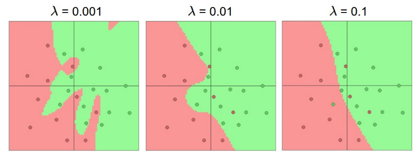
  → Smaller networks are harder to train with local methods such as Gradient Descent
  
  
• The regularization strength is the preferred way to control the overfitting of a neural network

The effects of regularization strength: Each neural network above has 20 hidden neurons, but changing the regularization strength makes its final decision regions smoother with a higher regularization.