[CS231n] 6. Neural Networks Part2 : Setting up the Data

preprocessing, weight initialization, batch normalization, regularization (L2/dropout)

 

1) Data Preprocessing

We will assume matrix X is of size [N x D] (N is the number of data, D is their dimensionality)

1.1) Mean subtraction

most common form of preprocessing

• Subtracting the mean across every individual feature in the data
• It has the geometric interpretation of centering the cloud of data around the origin along every dimension.
• X -= np.mean(X, axis = 0)


 

1.2) Normalization

normalizing the data dimensions so that they are of approximately the same scale.

• Divide each dimension by its standard deviation
  → zero-centered: (X /= np.std(X, axis = 0))
• Another form of preprocessing normalizes each dimension so that the min and max along the dimension is -1 and 1 respectively.

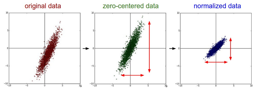
Common data preprocessing pipeline. Left: Original toy, 2-dimensional input data. Middle: The data is zero-centered by subtracting the mean in each dimension. The data cloud is now centered around the origin. Right: Each dimension is additionally scaled by its standard deviation. The red lines indicate the extent of the data - they are of unequal length in the middle, but of equal length on the right.

 

1.3) PCA

• The data is first centered as described above.
• Then, we can compute the covariance matrix that tells us about the correlation structure in the data

# Assume input data matrix X of size [N x D]
X -= np.mean(X, axis = 0) # zero-center the data (important)
cov = np.dot(X.T, X) / X.shape[0] # get the data covariance matrix

• The (i, j) element of the data covariance matrix contains the covariance between i-th and j-th dimension of the data.
• We can compute the SVD factorization of the data covariance matrix

U,S,V = np.linalg.svd(cov)

The columns of U are the eigenvectors and S is a 1-D array of the singular values. To decorrelate the data, we project the original (but zero-centered) data into the eigenbasis

Xrot = np.dot(X, U) # decorrelate the data

• the columns of U are a set of orthonormal vectors (norm of 1, and orthogonal to each other)
• The projection therefore corresponds to a rotation of the data in X so that the new axes are the eigenvectors.
• If we were to compute the covariance matrix of Xrot, we would see that it is now diagonal.
• A nice property of np.linalg.svd is that in its returned value U, the eigenvector columns are sorted by their eigenvalues.
  → We can use this to reduce the dimensionality of the data by only using the top few eigenvectors, and discarding the dimensions along which the data has no variance.

Xrot_reduced = np.dot(X, U[:,:100]) # Xrot_reduced becomes [N x 100]

• After this operation, we would have reduced the original dataset of size [N x D] to one of size [N x 100], keeping the 100 dimensions of the data that contain the most variance.
  → good performance by training linear classifiers or neural networks on the PCA-reduced datasets, obtaining savings in both space and time.

 

1.4) Whitening

Takes the data in the eigenbasis and divides every dimension by the eigenvalue to normalize the scale.

• The geometric interpretation of this transformation is that if the input data is a multivariable gaussian, then the whitened data will be a gaussian with zero mean and identity covariance matrix.

# whiten the data:
# divide by the eigenvalues (which are square roots of the singular values)
Xwhite = Xrot / np.sqrt(S + 1e-5)

• Warning : Exaggerating noiseOne weakness of this transformation is that it can greatly exaggerate the noise in the data
• we’re adding 1e-5 (or a small constant) to prevent division by zero.

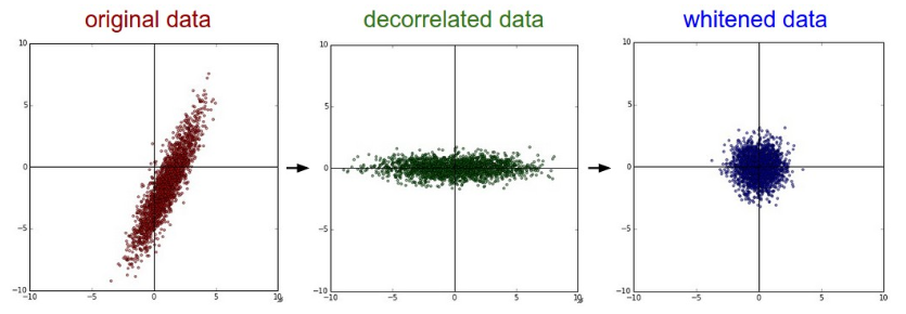
PCA / Whitening. Left: Original toy, 2-dimensional input data. Middle: After performing PCA. The data is centered at zero and then rotated into the eigenbasis of the data covariance matrix. This decorrelates the data (the covariance matrix becomes diagonal). Right: Each dimension is additionally scaled by the eigenvalues, transforming the data covariance matrix into the identity matrix. Geometrically, this corresponds to stretching and squeezing the data into an isotropic gaussian blob.

 

Left :An example set of 49 images.

2nd from Left: The top 144 out of 3072 eigenvectors. The top eigenvectors account for most of the variance in the data, and we can see that they correspond to lower frequencies in the images.

2nd from Right: The 49 images reduced with PCA, using the 144 eigenvectors shown here. That is, instead of expressing every image as a 3072-dimensional vector where each element is the brightness of a particular pixel at some location and channel, every image above is only represented with a 144-dimensional vector, where each element measures how much of each eigenvector adds up to make up the image. In order to visualize what image information has been retained in the 144 numbers, we must rotate back into the "pixel" basis of 3072 numbers. Since U is a rotation, this can be achieved by multiplying by U.transpose()[:144,:], and then visualizing the resulting 3072 numbers as the image. You can see that the images are slightly blurrier, reflecting the fact that the top eigenvectors capture lower frequencies. However, most of the information is still preserved.

Right: Visualization of the "white" representation, where the variance along every one of the 144 dimensions is squashed to equal length. Here, the whitened 144 numbers are rotated back to image pixel basis by multiplying by U.transpose()[:144,:]. The lower frequencies (which accounted for most variance) are now negligible, while the higher frequencies (which account for relatively little variance originally) become exaggerated.

• In practice, these transformations are not used with Convolutional Networks. However, it is very important to zero-center the data, and it is common to see normalization of every pixel as well.

 

2) Weight Initialization

Before we can begin to train the network we have to initialize its parameters.

• Pitfall: all zero initialization
  If every neuron in the network computes the same output, then they will also all compute the same gradients during backpropagation and undergo the exact same parameter updates.
  → we should not do
  
  
• Small random numbers
  The neurons are all random and unique in the beginning, so they will compute distinct updates and integrate themselves as diverse parts of the full network.
  The implementation for one weight matrix might look like W = 0.01* np.random.randn(D, H), where randn samples from a zero mean, unit standard deviation gaussian.
  → This seems to have relatively little impact on the final performance in practice.
  
  
• Calibrating the variances with 1/sqrt(n)
  We can normalize the variance of each neuron’s output to 1 by scaling its weight vector by the square root of its fan-in (i.e. its number of inputs)
  The recommended heuristic is to initialize each neuron’s weight vector as: w = np.random.randn(n) / sqrt(n), where n is the number of its inputs.
  → This ensures that all neurons in the network initially have approximately the same output distribution and empirically improves the rate of convergence.
  
  
• He initialization
  Initialization specifically for ReLU neurons, reaching the conclusion that the variance of neurons in the network should be 2.0/n
  → w = np.random.randn(n) * sqrt(2.0/n), and is the current recommendation for use in practice in the specific case of neural networks with ReLU neurons.

 

3) Batch Normalization

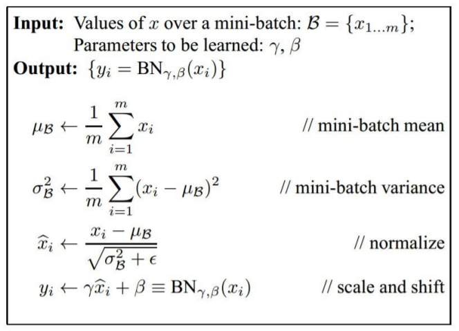
Properly initializing neural networks by explicitly forcing the activations throughout a network to take on a unit gaussian distribution at the beginning of the training.

• Applying this technique usually amounts to insert the BatchNorm layer immediately after fully connected layers (or convolutional layers), and before non-linearities.
• Use Batch Normalization are significantly more robust to bad initialization.
• Scale and Shift → increase flexibility

Pros

• Improves gradient flow through the network
• Allows higher learning rates
• Acts as a form of regularization in a funny way, and slightly reduces the need for dropout, maybe

 

4) Regularization

There are several ways of controlling the capacity of Neural Networks to prevent overfitting

• L2 regularization
  It can be implemented by penalizing the squared magnitude of all parameters directly in the objective.For every weight w in the network, we add the term 1/2*λw^2 to the objective, where λ is the regularization strength.
• L1 regularization
  Each weight w we add the term λ∣w∣ to the objective. The L1 regularization has the intriguing property that it leads the weight vectors to become sparse during optimization (i.e. very close to exactly zero).
  Neurons with L1 regularization end up using only a sparse subset of their most important inputs and become nearly invariant to the “noisy” inputs.

Final weight vectors from L2 regularization are usually diffuse, small numbers. In practice, if you are not concerned with explicit feature selection, L2 regularization can be expected to give superior performance over L1.

4.1) Dropout

Extremely effective, simple and recently introduced regularization technique

• While training, dropout is implemented by only keeping a neuron active with some probability p (a hyperparameter), or setting it to zero otherwise.

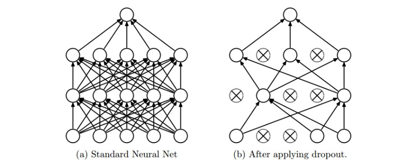
During training, Dropout can be interpreted as sampling a Neural Network within the full Neural Network, and only updating the parameters of the sampled network based on the input data. (However, the exponential number of possible sampled networks are not independent because they share the parameters.) During testing there is no dropout applied, with the interpretation of evaluating an averaged prediction across the exponentially-sized ensemble of all sub-networks (more about ensembles in the next section).

• Vanilla dropout in an example 3-layer Neural Network would be implemented as follows

""" Vanilla Dropout: Not recommended implementation (see notes below) """

p = 0.5 # probability of keeping a unit active. higher = less dropout

def train_step(X):
  """ X contains the data """

  # forward pass for example 3-layer neural network
  H1 = np.maximum(0, np.dot(W1, X) + b1)
  U1 = np.random.rand(*H1.shape) < p # first dropout mask
  H1 *= U1 # drop!
  H2 = np.maximum(0, np.dot(W2, H1) + b2)
  U2 = np.random.rand(*H2.shape) < p # second dropout mask
  H2 *= U2 # drop!
  out = np.dot(W3, H2) + b3

  # backward pass: compute gradients... (not shown)
  # perform parameter update... (not shown)

def predict(X):
  # ensembled forward pass
  H1 = np.maximum(0, np.dot(W1, X) + b1) * p # NOTE: scale the activations
  H2 = np.maximum(0, np.dot(W2, H1) + b2) * p # NOTE: scale the activations
  out = np.dot(W3, H2) + b3

• Inside the train_step function we have performed dropout twice: on the first hidden layer and on the second hidden layer.
• In the predict function we are not dropping anymore, but we are performing a scaling of both hidden layer outputs by p.
  
  
• test-time performance is so critical, it is always preferable to use inverted dropout, which performs the scaling at train time, leaving the forward pass at test time untouched.

""" 
Inverted Dropout: Recommended implementation example.
We drop and scale at train time and don't do anything at test time.
"""

p = 0.5 # probability of keeping a unit active. higher = less dropout

def train_step(X):
  # forward pass for example 3-layer neural network
  H1 = np.maximum(0, np.dot(W1, X) + b1)
  U1 = (np.random.rand(*H1.shape) < p) / p # first dropout mask. Notice /p!
  H1 *= U1 # drop!
  H2 = np.maximum(0, np.dot(W2, H1) + b2)
  U2 = (np.random.rand(*H2.shape) < p) / p # second dropout mask. Notice /p!
  H2 *= U2 # drop!
  out = np.dot(W3, H2) + b3

  # backward pass: compute gradients... (not shown)
  # perform parameter update... (not shown)

def predict(X):
  # ensembled forward pass
  H1 = np.maximum(0, np.dot(W1, X) + b1) # no scaling necessary
  H2 = np.maximum(0, np.dot(W2, H1) + b2)
  out = np.dot(W3, H2) + b3

• In practice
  It is also common to combine this with dropout applied after all layers.
  It is most common to use a single, global L2 regularization strength that is cross-validated.
  → The value of p=0.5 is a reasonable default, but this can be tuned on validation data.
  
  

4.2) Data Augmentation

• It is used in their experiments to increase the dataset size
• Horizontal Flips

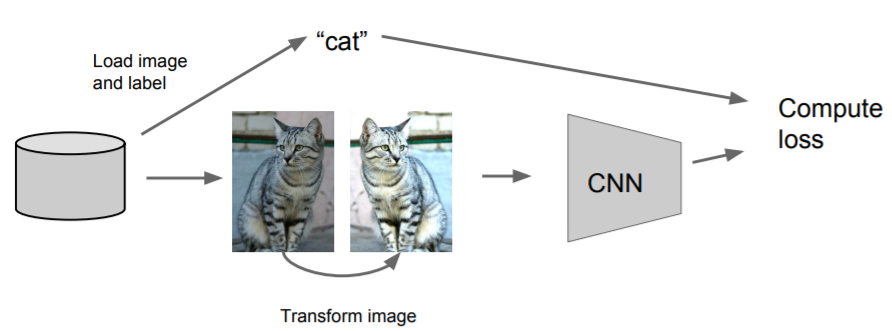
• Random crops and scales
• Color Jitter / Randomize contrast and brightness
• Random mix/combinations of :
• translation, rotation, stretching, shearing, lens distortions,..

Regularization : A common pattern

• Training : Add random noise
• Testing : Marginalize over the noise
• Examples : Dropout, Batch Normalization, Data Augmentation, DropConnect, Fractional Max Pooling, Stochastic Depth