[CS231n] 9. Convolutional Neural Networks: Layer Patterns, Case studies

ConvNet Architectures

We have seen that Convolutional Networks are commonly made up of only three layer types: CONV, POOL and FC. We will also explicitly write the ReLU activation function as a layer, which applies elementwise non-linearity.

 

Layer Patterns

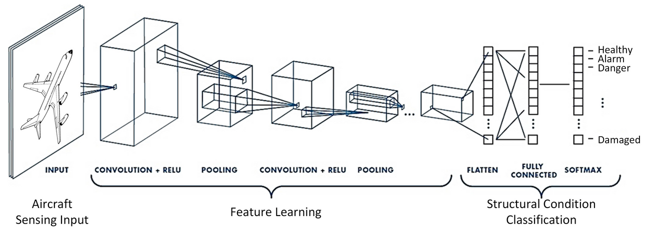
The most common form of a ConvNet architecture stacks a few CONV-ReLU layers, follows them with POOL layers, and repeats this pattern until the image has been merged spatially to a small size. The last FC layer holds the output, such as the class scores.

• INPUT -> [[CONV -> RELU]*N -> POOL?]*M -> [FC -> RELU]*K -> FC
  → where the * indicates repetition, and the POOL? indicates an optional pooling layer. Moreover, N >= 0 (and usually N <= 3), M >= 0, K >= 0 (and usually K < 3).

Some common ConvNet architectures

• INPUT -> FC, implements a linear classifier. Here N = M = K = 0.
• INPUT -> CONV -> ReLU -> FC
• INPUT -> [CONV -> ReLU -> POOL]*2 -> FC -> ReLU -> FC. Here we see that there is a single CONV layer between every POOL layer.
• INPUT -> [CONV -> ReLU -> CONV -> ReLU -> POOL]*3 -> [FC -> ReLU]*2 -> FC Here we see two CONV layers stacked before every POOL layer. This is generally a good idea for larger and deeper networks, because multiple stacked CONV layers can develop more complex features of the input volume before the destructive pooling operation.

 

Prefer a stack of small filter CONV to one large receptive field CONV layer.

• Suppose that you stack three 3x3 CONV layers on top of each other (with non-linearities in between).
  → Each neuron on the first CONV layer has a 3x3 view of the input volume. A neuron on the second CONV layer has a 3x3 view of the first CONV layer, and hence by extension a 5x5 view of the input volume.
  → Similarly, a neuron on the third CONV layer has a 3x3 view of the 2nd CONV layer, and hence a 7x7 view of the input volume.
• Suppose that instead of these three layers of 3x3 CONV, we only wanted to use a single CONV layer with 7x7 receptive fields.
• Several disadvantages
  1. The neurons would be computing a linear function over the input, while the three stacks of CONV layers contain non-linearities that make their features more expressive.
  2. If we suppose that all the volumes have C channels, then it can be seen that the single 7x7 CONV layer would contain C×(7×7×C)=49C^2 parameters, while the three 3x3 CONV layers would only contain 3×(C×(3×3×C))=27C^2 parameters.
     → Stacking CONV layers with tiny filters as opposed to having one CONV layer with big filters allows us to express more powerful features of the input, and with fewer parameters.

 

Recent departures

The conventional paradigm of a linear list of layers has recently been challenged

• In Google’s Inception architectures and also in current (state of the art) Residual Networks from Microsoft Research Asia.
• Both of these feature more intricate and different connectivity structures.

 

---

 

Layer Sizing Patterns

• The input layer (that contains the image) should be divisible by 2 many times.
  → Common numbers include 32 (e.g. CIFAR-10), 64, 96 (e.g. STL-10), or 224 (e.g. common ImageNet ConvNets), 384, and 512.

• The conv layers should be using small filters (e.g. 3x3 or at most 5x5), using a stride of S=1, and crucially, padding the input volume with zeros in such way that the conv layer does not alter the spatial dimensions of the input.
• The pool layers are in charge of downsampling the spatial dimensions of the input. The most common setting is to use max-pooling with 2x2 receptive fields (i.e. F=2), and with a stride of 2 (i.e. S=2).
  → this discards exactly 75% of the activations in an input volume (due to downsampling by 2 in both width and height).

 

Why use stride of 1 in CONV?

Smaller strides work better in practice. Additionally, as already mentioned stride 1 allows us to leave all spatial down-sampling to the POOL layers, with the CONV layers only transforming the input volume depth-wise.

 

Why use padding?

In addition to the aforementioned benefit of keeping the spatial sizes constant after CONV, doing this actually improves performance. If the CONV layers were to not zero-pad the inputs and only perform valid convolutions, then the size of the volumes would reduce by a small amount after each CONV, and the information at the borders would be “washed away” too quickly.

 

Case Studies

There are several architectures in the field of Convolutional Networks that have a name.

 

1. LeNet

The first successful applications of Convolutional Networks were developed by Yann LeCun in 1990’s

 

2. AlexNet

The first work that popularized Convolutional Networks in Computer Vision

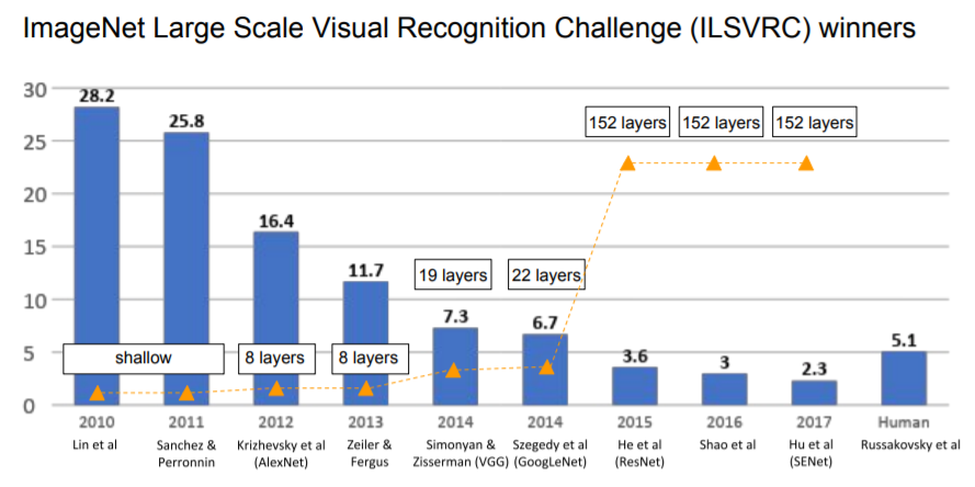
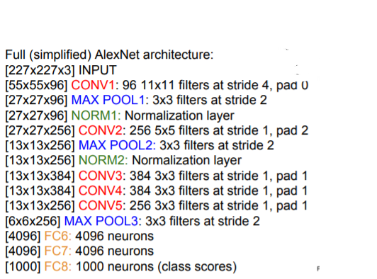
• The AlexNet was submitted to the ImageNet ILSVRC challenge in 2012 and significantly outperformed the second runner-up (top 5 error of 16% compared to runner-up with 26% error)
• The Network had a very similar architecture to LeNet, but was deeper, bigger, and featured Convolutional Layers stacked on top of each other (previously it was common to only have a single CONV layer always immediately followed by a POOL layer)

 

 

Details / Retrospectives

• First use of ReLU
• Used Norm layers(not common anymore)
• heavy data argumentation
• dropout 0.5
• batch size 128
• SGD Momentum 0.9
• Learning rate 1e-2, reduced by 10 manually when val accuracy plateaus
• L2 weight decay 5e-4
• 7 CNN ensemble: 18.2% → 15.4%

 

3. ZF Net

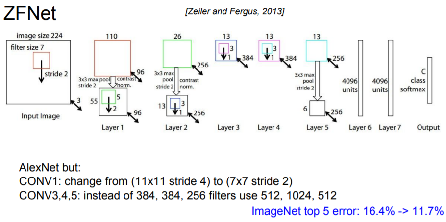
The ILSVRC 2013 winner was a Convolutional Network from Matthew Zeiler and Rob Fergus.(short for Zeiler & Fergus Net)

• It was an improvement on AlexNet by tweaking the architecture hyperparameters
• In particular by expanding the size of the middle convolutional layers and making the stride and filter size on the first layer smaller.

 

4. GoogLeNet

The ILSVRC 2014 winner was a Convolutional Network from Szegedy et al. from Google.

• Its main contribution was the development of an Inception Module that dramatically reduced the number of parameters in the network (4M, compared to AlexNet with 60M)
• Its main contribution was the development of an Inception Module that dramatically reduced the number of parameters in the network (4M, compared to AlexNet with 60M)

• Inception module : design a good local network topology(network within a network) and then stack these modules on top of each other

→ bottleneck layers that use 1x1 convolutions to reduce feature depth

→ Auxiliary classification outputs to inject additional gradient at lower layers

 

5. VGGNet

The runner-up in ILSVRC 2014 was the network from Karen Simonyan and Andrew Zisserman that became known as the VGGNet.

• Its main contribution was in showing that the depth of the network is a critical component for good performance.
• Their final best network contains 16 CONV/FC layers and, appealingly, features an extremely homogeneous architecture that only performs 3x3 convolutions and 2x2 pooling from the beginning to the end.

• Stack of three 3x3 conv (stride 1) layers has same effective receptive field as one 7x7 conv layer
• → But deeper, more non-linearities and fewer parameters 3(3^2C^2) vs. 7^2*C^2 for C channels per layer

 

6. ResNet

Residual Network developed by Kaiming He et al. was the winner of ILSVRC 2015.

• It features special skip connections and a heavy use of batch normalization.
• The architecture is also missing fully connected layers at the end of the network.

 

Comparing complexity

• Inception-v4 : Resnet + Inception
• VGG : Highest memory, most operations
• GoogLeNet : most efficient
• AlexNet : Smaller compute, still memory heavy, lower accuracy
• ResNet : Moderate efficiency depending on model, highest accuracy

 

Summary

• VGG, GoogLeNet, ResNet all in wide use, available in model zoos
• ResNet current best default, also consider SENet when available
• Trend towards extremely deep networks
• Significant research centers around design of layer / skip connections and improving gradient flow
• Efforts to investigate necessity of depth vs. width and residual connections
• Even more recent trend towards meta-learning

​