[CS231n] 1. Image Classification

Keywords : Data-driven Approach, K-Nearest Neighbor, train/validation/test splits

L1,L2 distances, hyperparameter search, cross-validation

 

1. Image Classification

• The task of assigning an input image one label from a fixed set of categories
• One of the core problems in Computer Vision

1) Example

• A single image and assigns probabilities to 4 labels, {cat, dog, hat, mug}
• The cat image is 248 pixels wide, 400 pixels tall, and has three color(RGB) channels

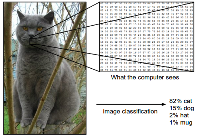
image consists of 248 x 400 x 3 numbers, or a total of 297,600 numbers

• Each number is an integer that ranges from 0 (black) to 255 (white).
• Our task is to turn this quarter of a million numbers into a single label, such as “cat”.

 

2) Challenges

1. Viewpoint variation : A single instance of an object can be oriented in many ways with respect to the camera
2. Scale variation : Visual classes often exhibit variation in their size
3. Deformation : Many objects of interest are not rigid bodies and can be deformed in extreme ways
4. Occlusion : The objects can be occluded. Sometimes a small portion of an object could be visible
5. Illumination conditions : The effects of illumination are drastic on the pixel level
6. Background clutter : The objects of interest may blend into their environment, making them hard to identify
7. Intra-class variation : The classes of interest can often be relatively broad, such as chair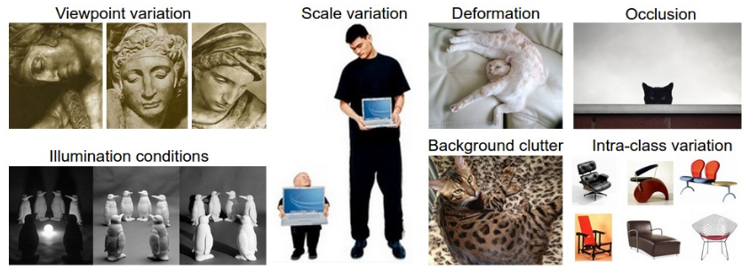

→ A good image classification model must be invariant to the cross product of all these variations, while simultaneously retaining sensitivity to the inter-class variations.

 

3) Data-driven Approach

• Develop learning algorithms that look at many examples and learn about the visual appearance of each class

An example training set for four visual categories

1. Collect a dataset of images and labels
2. Use Machine Learning to train a classifier
3. Evaluate the classifier on new images

 

4) The Image Classification Pipeline

• Input
  • Input consists of a set of N images, each labeled with one of K different classes.
  • We refer to this data as the training set.
• Learning
  • Task is to use the training set to learn what every one of the classes looks like.
  • We refer to this step as training a classifier, or learning a model
• Evaluation
  • Evaluate the quality of the classifier by asking it to predict labels for a new set of images that it has never seen before. Then, compare the true labels of these images to the ones predicted by the classifier. Hope that a lot of the predictions match up with the true answers(ground truth).

 

 

---

 

2. Nearest Neighbor Classifier

It is very rarely used in practice, but it will allow us to get an idea about the basic approach to an image classification problem.

1. Memorize all data and labels
2. Predict the label of the most similar training image

 

1) Example

• Image classification dataset: CIFAR-10
  • This dataset consists of 60,000 tiny images that are 32 pixels high and wide. Each image is labeled with one of 10 classes
  • One popular toy image classification dataset is the CIFAR-10 dataset.

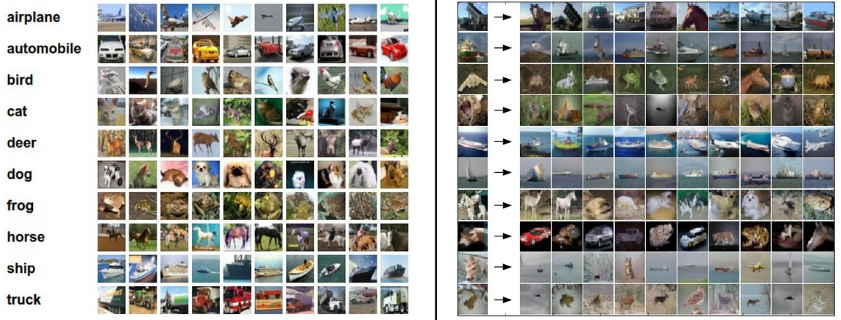
Left: Example images from the CIFAR-10 dataset. Right: first column shows a few test images and next to each we show the top 10 nearest neighbors in the training set according to pixel-wise difference.

• One of the simplest possibilities is to compare the images pixel by pixel and add up all the differences.
• Given two images and representing them as vectors I1,I2 , a reasonable choice for comparing them might be the L1 distance:

An example of using pixel-wise differences to compare two images with L1 distance (for one color channel in this example)

 

 

2) Implement the classifier in code

• Load the CIFAR-10 data into memory as 4 arrays

Xtr, Ytr, Xte, Yte = load_CIFAR10('data/cifar10/') # a magic function we provide 
# flatten out all images to be one-dimensional 
Xtr_rows = Xtr.reshape(Xtr.shape[0], 32 * 32 * 3) # Xtr_rows becomes 50000 x 3072 
Xte_rows = Xte.reshape(Xte.shape[0], 32 * 32 * 3) # Xte_rows becomes 10000 x 3072

- Xtr (of size 50,000 x 32 x 32 x 3) holds all the images in the training set

- Ytr (of length 50,000) holds the training labels (from 0 to 9)

 

• Here is how we could train and evaluate a classifier:

nn = NearestNeighbor() # create a Nearest Neighbor classifier class 
nn.train(Xtr_rows, Ytr) # train the classifier on the training images and labels 
Yte_predict = nn.predict(Xte_rows) # predict labels on the test images 
# and now print the classification accuracy, which is the average number 
# of examples that are correctly predicted (i.e. label matches) 
print('accuracy: %f' % ( np.mean(Yte_predict == Yte) ))

Notice that as an evaluation criterion, it is common to use the accuracy, which measures the fraction of predictions that were correct.

- train(X,y) function takes the data and the labels to learn.

- predict(X) function takes new data and predicts the labels.

 

• Implementation of a simple Nearest Neighbor classifier with the L1 distance:

import numpy as np 

class NearestNeighbor(object): 
	def __init__(self): 
		pass 
    
    def train(self, X, y): 
    """ X is N x D where each row is an example. Y is 1-dimension of size N """ 
    # the nearest neighbor classifier simply remembers all the training data 
    self.Xtr = X 
    self.ytr = y 
    
    def predict(self, X): 
    """ X is N x D where each row is an example we wish to predict label for """ 
    num_test = X.shape[0] 
    # lets make sure that the output type matches the input type 
    Ypred = np.zeros(num_test, dtype = self.ytr.dtype) 
    
    # loop over all test rows 
    for i in range(num_test): 
    	# find the nearest training image to the i'th test image 
        # using the L1 distance (sum of absolute value differences) 
        distances = np.sum(np.abs(self.Xtr - X[i,:]), axis = 1) 
        min_index = np.argmin(distances) # get the index with smallest distance 
        Ypred[i] = self.ytr[min_index] # predict the label of the nearest example 
        
     return Ypred

If you ran this code, you would see that this classifier only achieves 38.6% on CIFAR-10. That’s more impressive than guessing at random (which would give 10% accuracy)

• Q. With N examples, how fast are training and prediction?
  • A. Train O(1), Predict O(N)
  • This is bad : we want classifiers that are fast at prediction; slow for training is ok

 

3) The choice of distance

• L2 distance
  • It has the geometric interpretation of computing the euclidean distance between two vectors.

 

4) L1(Manhattan distance) vs. L2(Euclidean distance)

The L2 distance is much more unforgiving than the L1 distance when it comes to differences between two vectors.

• Manhattan distance vs. Euclidean distance
  • In Manhattan distance, the red, yellow, and blue paths all have the same shortest path length of 12. In Euclidean geometry, the green line has length and is the unique shortest path.

 

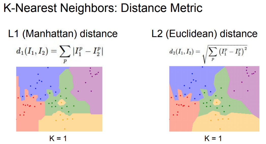
Compared to L2, L1 has many classification lines parallel to the axis.

The L2 distance shows a consistent circle regardless of the axes. This can be interpreted as showing that the L1 distance is more affected by the shape of the input data than the L2 distance.

 

---

 

3. K-Nearest Neighbor Classifier & Code with Google Colab

• Take majority vote from K closest points
• Intuitively, higher values of k have a smoothing effect that makes the classifier more resistant to outliers

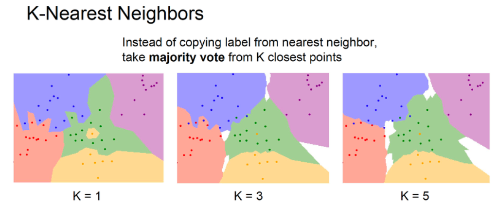
In NN classifier, outlier datapoints (e.g. yellow point in the middle of a cloud of green points) create small islands of likely incorrect predictions, while the 5-NN classifier smooths over these irregularities, likely leading to better generalization on the test data.

 

Running K-NN Code with Google Colab

 

---

 

4. Validation sets for Hyperparameter tuning

The k-nearest neighbor classifier requires a setting for k. But what number works best? Additionally, we saw that there are many different distance functions we could have used: L1 norm, L2 norm..

These choices are called hyperparameters

• We cannot use the test set for the purpose of tweaking hyperparameters.
• You may tune your hyperparameters to work well on the test set, but if you were to deploy your model you could see a significantly reduced performance.
  • We would say that you overfit to the test set
• There is a correct way of tuning the hyperparameters. The idea is to split our training set in two
  • a slightly smaller training set, and what we call a validation set.

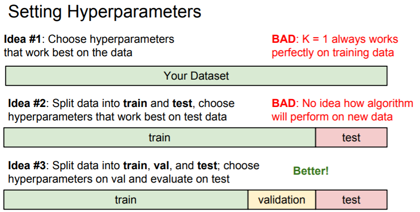
Split training set into training set and a validation set. Use validation set to tune all hyperparameters. At the end run a single time on the test set and report performance.

 

1) Cross-Validation

In 5-fold cross-validation, we would split the training data into 5 equal folds, use 4 of them for training, and 1 for validation. We would then iterate over which fold is the validation fold, evaluate the performance, and finally average the performance across the different folds.

• In practice, people prefer to avoid cross-validation in favor of having a single validation split, since cross-validation can be computationally expensive.

 

2) Pros & Cons of Nearest Neighbor Classifier

Pros

• It is very simple to implement and understand
• The classifier takes no time to train, since all that is required is to store and possibly index the training data.

Cons

• We pay that computational cost at test time, since classifying a test example requires a comparison to every single training example.
• Images are high-dimensional objects (i.e. they often contain many pixels), and distances over high-dimensional spaces can be very counter-intuitive.

Pixel-based distances on high-dimensional data (and images especially) can be very unintuitive. An original image (left) and three other images next to it that are all equally far away from it based on L2 pixel distance. Clearly,  the pixel-wise distance does not correspond at all to perceptual or semantic similarity .

 

We saw that the use of L1 or L2 distances on raw pixel values is not adequate since the distances correlate more strongly with backgrounds and color distributions of images than with their semantic content.